Chanel Belvin, Toni Dunlap, Jimmy Newland, & Elaine Soares
Monday, June 15, 2 pm – San Felipe A & B
STEM Educator and Researcher.
Chanel Belvin, Toni Dunlap, Jimmy Newland, & Elaine Soares
Monday, June 15, 2 pm – San Felipe A & B
Tuesday, June 16, 2026, 11:15am – 12:15pm CDT; San Augustine B – 3rd Floor
Be sure to visit my GitHub repository for my collection of computational essays as curricular tools.
Data science pedagogy can enhance learning experiences for students across all STEM courses, regardless of traditional data science use. Come learn how to integrate data storytelling directly into your class. This session will provide you with resources that you can implement right away in your classroom.

Be sure to visit the Cepheus C YSO Catalog Creation project page to see details about our iPoster presentation at AAS 247 in Phoenix, Arizona, 4-8 January, 2026.

Houston Astronomical Society December 5th, 2025
Modern astronomy research has become data-driven. Using data science techniques alongside computation allows us to interrogate data to understand astrophysical phenomena. The explosion of data sets has opened up new ways for enterprising amateur astronomers to contribute to modern astronomical research. Data can come from large-scale surveys, space-based observatories, individual scientists, or students. You can learn to select, reduce, visualize, and interpret authentic astronomical data while applying data science techniques to construct astronomy knowledge. Many free web-based tools leverage data science techniques. This talk explores how these activities bridge the gap between data science and astronomy, enabling amateurs to learn about both simultaneously.
The content of this talk can be cited as: Newland, J. (2025). Using Data Science in High School Astronomy. ASP 2024: Astronomy Across the Spectrum, 539, 147. http://arxiv.org/abs/2501.04856
The Google Colab (Jupyter Notebook) developed by Sara Kannan and me can be found here. Note that the actual catalog we created is not publicly available, so this notebook requires an existing catalog for SED creation.
If you are interested in data-driven astronomy learning, check out the page below from a talk given at the first-ever Data Science Education in K12 Conference. Even though the materials shared were designed for teaching high school astronomy, enterprising amateur astronomers can still pick up some cool tricks.
CAST 2025
Jimmy Newland and Justin Hickey
Zoom link (just in case!)
Choose your own adventure!
If you are interested in the role of data science pedagogy in teaching science, check out this page.
When doing domain-specific programming in science, some CS pedagogy can be used to
scaffold concepts like conditionals, function writing, and looping. Using worked examples,
minimally working programs, sub-task labeling, and live coding can help a student bring
coding to bear on learning concepts in science. Room B107 1:15 – 2:15 pm CDT
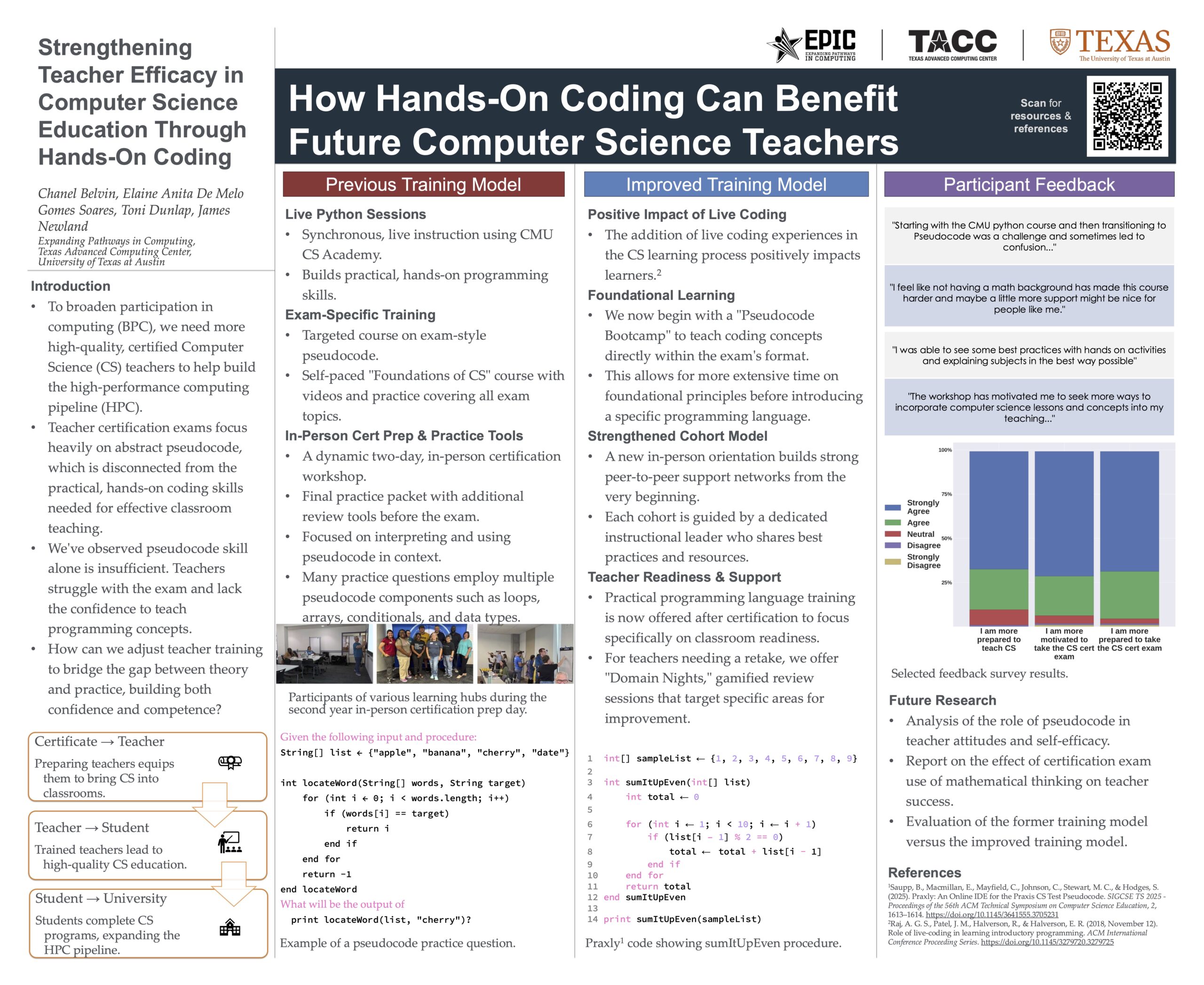
Chanel Belvin, Elaine Anita De Melo Gomes Soares, Toni Dunlap, James Newland
Expanding Pathways in Computing,
Texas Advanced Computing Center,
University of Texas at Austin