Photometric Catalog Integration in a Python Framework for Spectral Energy Distribution Construction and Young Stellar Object Classification

James Newland (1), Sara Kannan (2), Luisa Rebull (3)
Texas Advanced Computing Center University of Texas at Austin (1), Bellaire Senior High School (2), Infrared Science Archive IPAC California Institute of Technology (3)

Abstract
One method for studying young stellar objects (YSOs) is by assembling their spectral energy distributions (SEDs) from
multi-wavelength photometric catalogs. These SEDs can be used to estimate the relative ages of YSOs. In the Cepheus C
region, we took an existing photometric catalog created using both infrared and visible data from 2MASS, Spitzer,
WISE, Herschel, SDSS, IPHAS, and PanSTARRS missions, and updated the catalog using data from the Gaia survey.
We focused on constructing SEDs and using their shapes for preliminary classification. To support this effort, we
developed a Python-based Google Colab notebook that implements SED construction using tools such as Astropy,
Astroquery, and pandas. While generating SED plots can be computationally straightforward with a completed notebook, verifying catalog matches and cleaning legacy data is labor-intensive and critical to data integrity. The notebook is meant as a part of the process of teaching students to access, manipulate, visualize, and explain astronomical datasets. Our pipeline is designed to help students engage with real astronomical data, emphasizing transparency in data handling and reproducibility. The use of a computational essay format allows for narrative text and code blocks to co-exist in a single structure. This work is part of a broader educational initiative to involve high school students in authentic research through computational essays in Google Colab. We followed best practices in data science education, including the statistical problem-solving process, and structured our notebook to be accessible and reusable for other teams. Preliminary results from Cepheus C will be shared, along with suggestions for extending the catalog with time-series data to explore YSO variability, contributing to the larger YOSVAR project.
Background
Introduction
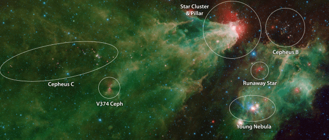
Cepheus C is a star-forming region within the larger Cepheus molecular cloud. We used archival photometric data to generate spectral energy distributions (SEDs) for young stellar objects (YSOs) identified in the literature and by a previous NITARP (NASA/IPAC Teacher Archive Research Program) team. Our analysis was compared to other NITARP groups.
The primary feature of our work is the creation of a Python-based pipeline for generating SEDs. Since our notebook is written as a computational essay, it is easy to understand regardless of one’s experience with computer science, data science, and programming. Since our notebook shows how the SEDs are created and can be easily manipulated, it will allow educators and students to contribute to genuine astronomy research. The use of Python and Jupyter Notebook-style tools is becoming part of introductory science coursework (2,3,4).
This is also a shift within the NITARP community, which has been using Excel and IDL for SED generation. Since
Python is much more prevalent in research and more useful, introducing educators to Python in this format and allowing them to play with the notebook equips them with vital computational and research skills. Bringing computation and data science to introductory astronomy courses means allowing students to learn astronomy in much the same way current astronomers do their work(2).
Previous Work
Two other NITARP teams have studied the Cepheus C region: CephC-LABS (5) and LLAMMa (6). It was also a target of the YSOVAR (7) time series monitoring program. Since this region already had a multi-wavelength catalog and classification for 114 YSOs, it was an ideal cluster to begin developing a Python-based pipeline. It was also an opportunity to update the 2017 catalog with new photometry data. We added Gaia data and searched the literature for additional YSOs and catalogs.
Our notebook is based in part on code written in IDL by Dr. Rebull, as well as the “Make an SED for YSOs in IC417 (8)” notebook created by the BINAP NITARP team; however, our tool is better for generating SEDs for an entire cluster at once.
Spectral Energy Distributions and Photometric Data
SEDs are plots of energy density as a function of wavelength. It is, in some sense, another representation of how bright
an object is as a function of wavelength. We can include photometric data from multiple telescopes in an SED. Many
large-scale or all-sky surveys provide publicly accessible photometry. Blackbodies often approximate stellar
photospheres. SEDs of stars plus circumstellar gas and dust do not look like blackbodies. (7).

What are Young Stellar Objects?
Stars form starting from large clouds of gas and dust, ending up as hydrogen-burning young stars on the main sequence. We use the term young stellar objects (YSOs) to encompass all of these stages of star formation. YSOs are typically surrounded by gas and dust, which intercept radiation from the central object and reradiate it in longer wavelengths. This re-radiation manifests in the SED as excess emission in the infrared (IR), or an IR excess.
A stellar photosphere can be approximated by a blackbody curve in an SED. A stellar photosphere with circumstellar
dust will have an IR excess. The evolution of YSOs has often been parameterized by fitting the SED between 2 and 25
microns. A rising SED, with more IR excess (Class I), is thought to be younger (more embedded) than a falling SED,
with less IR excess (Class II). The figure omits the Flat class, which was inserted between Class I and Class II to capture
the transition between rising and falling SEDs.

Developing Catalog and Python Notebook
Catalog Creation
Although a photometric catalog for Cepheus C existed, it had not been updated or reviewed for several years. We
included new Gaia data by fetching it from the NASA/IPAC IRSA database and merging it with the initial catalog using
TOPCAT (10). We also conducted a literature search for newer YSO targets and catalogs, and found none.
The addition of Gaia photometry enabled us to create updated spectral energy distributions and, to some extent, verify
SDSS data, which operated at similar wavelengths. However, since Gaia data are in the visible part of the spectrum, this
did not affect the classification of the YSOs. Future work may compare SED results from SDSS versus Gaia photometry.
Python Notebook
Our notebook (via GitHub) was written in a computational essay (4) format. We opted to
use Google Drive for catalog storage to make it easy for educators, students, and people of all experience levels, and to
avoid requiring local disk access. By using Google Colab (3), our notebook can be easily copied and edited to support
SED generation and/or YSO classification for any catalog.
The function of our notebook is to generate SEDs for each object in the catalog. Since we already had a CSV of
photometric data from previous NITARP teams, we uploaded our updated catalog (including Gaia) to our Google Drive.
This way, we could directly fetch the CSV in Google Colab.
Our initial catalog contained a lot of information, some of which would not be useful for creating spectral energy
distributions. An array was created containing the wavelengths and magnitudes needed for the SEDs. For this notebook,
we did not account for magnitude error or quality flags. Additionally, we chose to ignore upper limits.
The array measurements are converted to the correct units for SEDs (energy density).
Once the code-generated points are determined, we fit a Rayleigh-Jeans line to the model photosphere and fit a
regression line to them. Although SED classification is typically based on a linear fit (11) to all detections between 2 and
24 microns, we do two separate fits: one for 2 to 8 microns and one for 2 to 24 microns. This is because many of the
objects in our catalogs lack data beyond 8 microns, and the distribution of photometry across different wavelengths
varies. Linear regression fits were calculated for both 2 to 8 microns and 2 to 24 microns. The fit with the highest
Pearson correlation coefficient (R) was used in the classification process.

The points, Rayleigh-Jeans line, and regressions are plotted on an SED using Matplotlib (12), and each SED is added to a Google Drive folder.

A script uploads the SED images to a webpage for easier viewing. We also generated a few charts using Matplotlib
(12) to show the classification ratios for the objects we analyzed. This also helped us compare our results with past work
and see the difference between classification using points between 2 and 8 microns versus 2 and 24 microns.
In addition to being a more useful educational tool, our Python notebook is better for NITARP because it can classify
objects based on SEDs, which is not typically done by Excel-based teams. Using computational thinking (13) and data
science pedagogy (14) in the design of curricular artifacts means that science learning occurs more authentically.
Results and Analysis
Examples of SEDs
The following SEDs are a few of many that we generated, illustrating the variation in structure and classification. The numbers at the top right of each image correspond to the links on our website (https://cepsed.thinkingwithcode.com).

The image above is a good example of an SED produced by our notebook. There is an apparent infrared excess on the Rayleigh-Jeans side. We have many data points, and the slope of the regression line appears to be roughly the same when we use points between 2 and 8 um (2-8) and between 2 and 24 um (2-24).

Some of our SEDs’ linear fits, like the one shown above, yield drastically different classifications based on slope calculations between the 2-8 and 2-24 regression lines, driven by outliers. This object is Class III if we use only 2-8 microns, but Class I if we include the longer wavelength point. This illustrates that some of the limits marked in our original catalog may be incomplete. It also serves as an example of what could happen when we don’t have detections longer than 8 microns.
In our final output (CSV), we note whether there are differences between the 2-8 and 2-24 lines, and we calculate the R and R^2 values for each line to determine which provides the better fit for the object; however, we continue to use both regression lines because the R and R^2 values are not necessarily the best statistic for deciding which line to use. We also note objects that lack sufficient points for regression, likely due to limitations in the initial photometry.
Cluster Analysis

The plot above shows the implications of the regression method and compares our results with those of the YSOVAR/NITARP teams, who previously analyzed the region.
Based on our classification distribution, most of the stars in this region are later in development (Class II and Class III). We see very few protostars and Class I objects. Given the age of Cep C (1-5 Myr), the way the YSOs were selected (X-rays, IR excess), and the fact that stars spend more time in the later stages, it makes sense that we would find more Class II and Class III objects.
Future Goals
Our project is still in progress. Currently, we are working on…
- Generating a color magnitude diagram(CMD) of candidates in our catalog.
- Creating a notebook which is designed to pull data from any catalog using VO protocols and intended to be modified for use on other clusters or projects where mass-SED production is necessary (our current notebook can be modified, but since it was designed for use on Cep C, it might be difficult for an amateur, student, or educator to manipulate).
- Incorporating and double-checking all limits (currently, we are relying on limit markers from the catalog handed to us by previous NITARP teams).
- Pulling images from archives using VO protocols and Firefly.
- Creating classroom-usable versions of the computational essay tools.
In the future, we may choose to extend our work by…
Adding more data to our photometric catalog (ex. SPHEREx).
- Building and training a neural network to analyze the Rayleigh-Jeans side of SEDs rather than relying on the
arbitrary cut points for classifications, and in other words, taking into account more factors than slope. - Analyzing lightcurves for some of our YSO candidates.
- Producing a paper related to the catalog updates.
- Creation of classroom-ready activities based on this pipeline.
Disclosures
This research has made use of the NASA/IPAC Infrared Science Archive, which is funded by the National Aeronautics and Space Administration and operated by the California Institute of Technology.
Author Info
James (Jimmy) Newland is a Computer Science Education Specialist for EPIC (Expanding Pathways in Computing) at UT Austin’s Texas Advanced Computing Center (TACC), where he assists educators in learning computer science concepts and pedagogy to become certified computer science teachers. He holds a B.S. in physics and astronomy from Mississippi State University, as well as an M.Ed. and a Ph.D. in science education from the University of Houston. Jimmy is interested in exploring the integration of computer science and computational thinking into non-computing courses, as well as the impacts of participation in authentic computing research projects on students and teachers.
Sara Kannan is a high school senior at Bellaire High School in Bellaire, TX. She plans to major in electrical and computer engineering with a dream of designing scientific instruments for spacecraft, particularly space-based telescopes. In her free time, she enjoys working with animals, particularly cattle and dogs, as well as playing guitar, reading, building robots, and stargazing.
Dr. Luisa Rebull is an associate research scientist at Caltech in Pasadena, California, where she focuses on young, low-mass stars across our galaxy, using data from the Spitzer Space Telescope and other telescopes. She studies how they form, how their disks form and evolve, and how young stars and their disks change with time, specifically their rotation and accretion. Also, Dr. Rebull has worked with educators and their students on authentic astronomy research projects on young stellar objects for more than 15 years.
References
1 NASA/JPL-Caltech. (2025, December 19). Cepheus C and Cepheus B Region by Spitzer. https://science.nasa.gov/photojournal/cepheus-c-and-cepheus-b-region-by-spitzer-two-instrument/
2 Norman, D., Cruz, K., Desai, V., Lundgren, B., Bellm, E., Economou, F., Smith, A., Bauer, A., Nord, B., Schafer, C., Narayan, G., Li, T., Tollerud, E., Sipőcz, B., Stevance, H., Pickering, T., Sinha, M., Harrington, J., Kartaltepe, J., … Dong, C. (2019). The Growing Importance of a Tech Savvy Astronomy and Astrophysics Workforce. Bulletin of the AAS, 51(7). https://baas.aas.org/pub/2020n7i018
2 LaMee, A. (University of C. F. (2021). Teaching Science Content with Jupyter at Scale, Elementary Through University. American Association of Physics Teachers Virtual Winter Meeting 2021, 88–88. https://doi.org/10.48448/46br-xe05
3 Lundgren, B., & Trainor, R. (2023). ESCIP: A collaboration for developing and sharing educational Jupyter Notebooks. American Astronomical Society Meeting Abstracts, 241, 246.04. https://baas.aas.org/pub/2023n2i246p04/release/1
4 Odden, T. O. B., Silvia, D. W., & Malthe-Sørenssen, A. (2023). Using computational essays to foster disciplinary epistemic agency in undergraduate science. Journal of Research in Science Teaching, 60(5), 937–977. https://doi.org/10.1002/tea.21821
5 Evans, S., Rebull, L., Rutherford, T., Stalnaker, O., Taylor, J., Efsits, G., Harl, L., Keil, S., Learman, D., Leonard, L., & Russell, A. (2018). Searching for Young Stars in Cepheus C. American Astronomical Society Meeting Abstracts #231, 231, 339.02.
6 Orr, L., Rebull, L. M., Johnson, M., Miller, A., Aragon Orozco, A., Bakhaj, B., Bakshian, J., Chiffelle, E., DeLint, A., Gerber, S., Mader, J., Marengo, A., McAdams, J., Montufar, C., Orr, Q., San Emeterio, L., Stern, E., & Weisserman, D. (2017). Finding High Quality Young Star Candidates in Ceph C using X-ray, Optical, and IR data. American Astronomical Society Meeting Abstracts #229, 229, 241.10.
7 Rebull, L. M., Cody, A. M., Covey, K. R., Günther, H. M., Hillenbrand, L. A., Plavchan, P., Poppenhaeger, K., Stauffer, J. R., Wolk, S. J., Gutermuth, R., Morales-Calderón, M., Song, I., Barrado, D., Bayo, A., James, D., Hora, J. L., Vrba, F. J., Alves De Oliveira, C., Bouvier, J., … Guieu, S. (2014). Young stellar object variability (YSOVAR): Long timescale variations in the mid-infrared. Astronomical Journal, 148(5). https://doi.org/10.1088/0004-6256/148/5/92
8 Newland, J., Andreas, A., Hickey, J., Ramseyer, E., Strasburger, D., & Rebull, L. (2025). Bridging Research and the Classroom: Leveraging Multi-Wavelength Data for SED Plots of Young Stellar Objects Using Google Colab. American Astronomical Society Meeting Abstracts #245,245, 205.03.
9 Vallastro, CC BY-SA 4.0 <https://creativecommons.org/licenses/by-sa/4.0>, via Wikimedia Commons
10 Taylor, M. ~B. (2005). TOPCAT & STIL: Starlink Table/VOTable Processing Software. In P. Shopbell, M. Britton, & R. Ebert (Eds.), Astronomical Data Analysis Software and Systems XIV (Vol. 347, p. 29).
11 Virtanen, P., Gommers, R., Oliphant, T. E., Haberland, M., Reddy, T., Cournapeau, D., Burovski, E., Peterson, P., Weckesser, W., Bright, J., van der Walt, S. J., Brett, M., Wilson, J., Millman, K. J., Mayorov, N., Nelson, A. R. J., Jones, E., Kern, R., Larson, E., … van Mulbregt, P. (2020). SciPy 1.0: fundamental algorithms for scientific computing in Python. Nature Methods, 17(3), 261–272. https://doi.org/10.1038/s41592-019-0686-2
12 The Matplotlib Development Team. (2025). Matplotlib: Visualization with Python (v3.10.8). Zenodo. https://doi.org/10.5281/zenodo.17595503
13 Weintrop, D., Beheshti, E., Horn, M., Orton, K., Jona, K., Trouille, L., & Wilensky, U. (2016). Defining Computational Thinking for Mathematics and Science Classrooms. Journal of Science Education and Technology, 25(1), 127–147. https://doi.org/10.1007/s10956-015-9581-5
14 Bargagliotti, A., Franklin, C., Arnold, P., Johnson, S., Perez, L., Spangler, D. A., & Gould, R. (n.d.). Pre-K-12 Guidelines for Assessment and Instruction in Statistics Education II (GAISE II) A Framework for Statistics and Data Science Education Writing Committee The Pre-K-12 Guidelines for Assessment and Instruction. Retrieved July 4, 2024, from https://www.amstat.org/asa/files/pdfs/GAISE/GAISEIIPreK-12_Full.pdf